Decorrelation Stretching and Debunking the Black Dragon Canyon Pterosaur

February 2022

Background

In 1947, John Simonson chalked the outline of what he believed to be a pictograph of a “winged monster” in Black Dragon Canyon, Utah. Chalking is no longer allowed as it vandalizes the original painting and hinders accurate dating. Chalking and other destructive methods such as dosing pictographs with kerosene were done before modern archeological imaging methods to enhance the contrast of the paintings.

The chalk outline of John Simonson’s “winged monster” was controversial for decades as some researchers argued he had chalked several distinct pictographs together. It seemed that every person who attempted to decipher the rock art came to a different conclusion of what it portrays. The most infamous of these conclusions was by young earth creationists (YEC) who claim that the pictograph is of a living pterosaur. Typically, YEC use highly saturated images that make the pictograph seem like one solid drawing.

image from paper

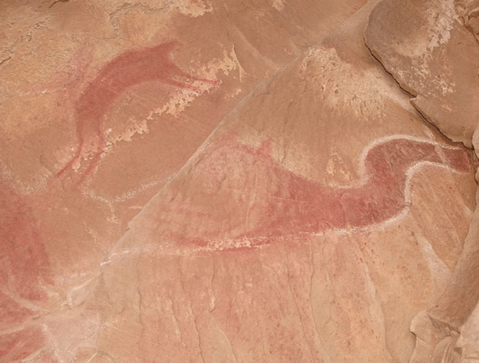
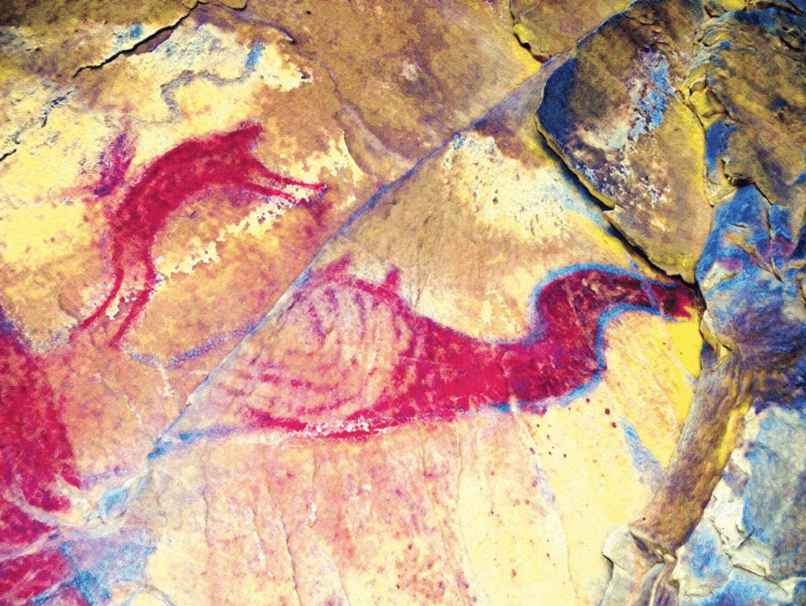
In 2013, researchers used a rock art enhancement plugin called DStretch to improve the visibility of the pictograph. They determined the paint was made with red ochre, which let them further filter the results to remove artifacts from the chalking and rock material. Using the DStretch results, they were able to reconstruct what it the original would have looked like by adjusting the color back to match the original red ochre and placing this back onto the rock wall.

paper results

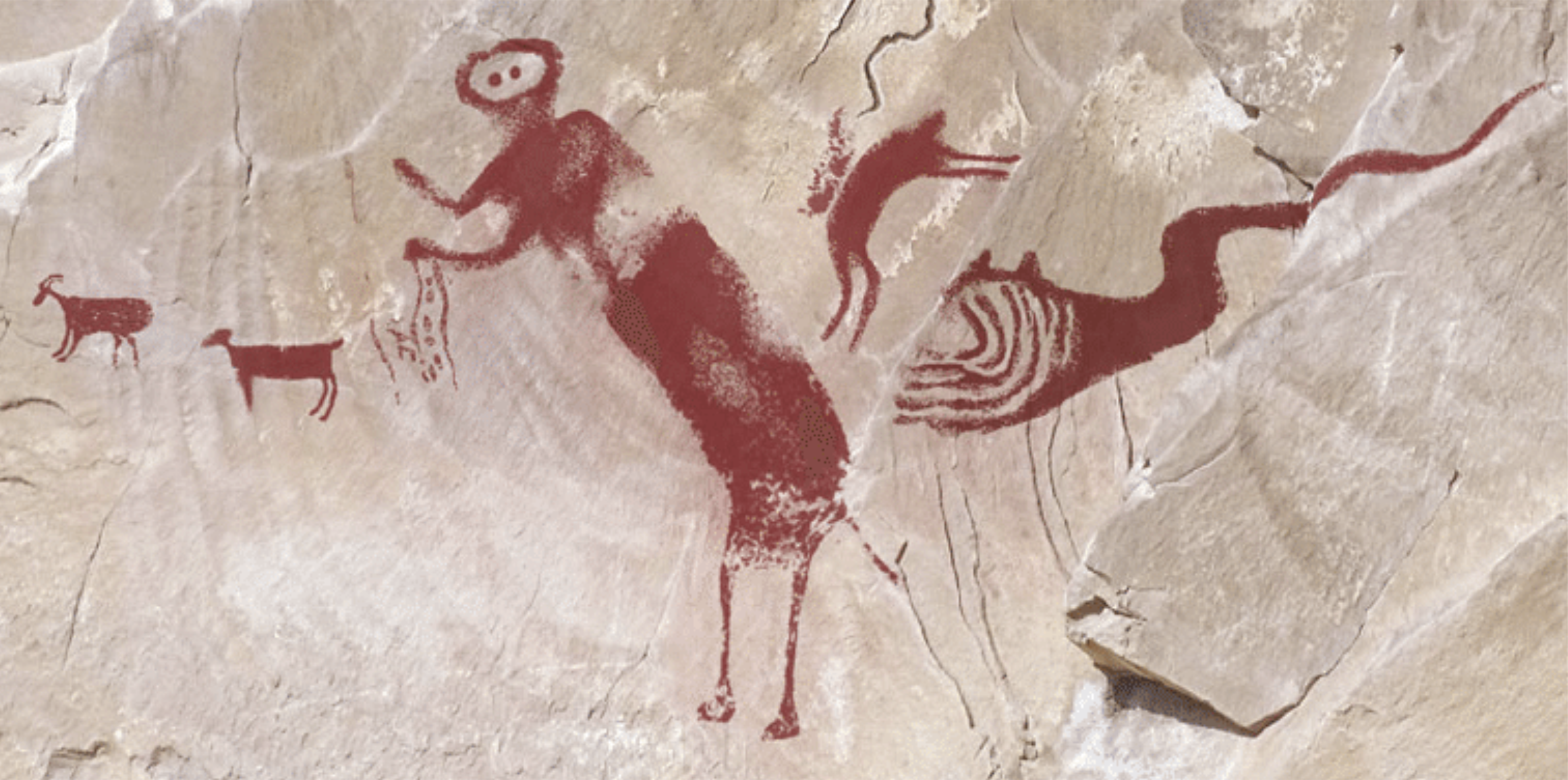
To further cement their results, the researchers used an X-ray fluorescence analyzer to compare the iron levels in the blank areas and the painted areas. Since the red ochre contains a high amount of iron, the painted areas showed high levels of iron while unpainted areas showed a low level. Their results aligned with the processed image, further bolstering the result.

Exploration of Decorrelation Stretch

I was curious how the DStretch plugin works, so I visited their website and discovered, unsurprisingly, it uses a method called decorrelation stretch. This method is used to enhance subtle color differences to make them more apparent to algorithms and the human eye. It’s used in hyperspectral imaging, aerial photography, and space photography (NASA’s Mars Rover used this method).

Decorrelation stretching and similar techniques such as the HSI transform seek to enhance images where the different channels (typically red, green, and blue) are highly correlated. This is done by exaggerating, or stretching, the saturation but not the lightness. These methods retain the original hue distribution, which is desirable. This can be seen in the rock art application as archeologists would want to retain the original hue distribution since the hues correspond to different pigments, rock material, and additions to the original like chalk.

Decorrelation stretching works by using PCA to project the image data to a space where it is no longer correlated (decorrelation). The result is then scaled according to some scheme (stretched), usually to equalize the variance, and projected back to the original image space.

Mathematically, the linear operation can be described by:

\[b_n=T*(a_n-\mu)+\mu_{target}\]

Where:

\(a_n\) and \(b_n\) are the RGB vectors for each pixel \(n\) in input image \(A\) and output image \(B\).
\(\mu\) is a vector of the means for each channel in the image \([\mu_R, \mu_B, \mu_G]\)
\(\mu_{target}\) is the desired output mean (typically equal to \(\mu\))
\(T\) is the linear transformation \(\sigma_{target}*V*S*V’\) where:
- \(\sigma_{target}\) is the desired output standard deviation (typically equal to \(\sigma\), the standard deviation of each band \([\sigma_R, \sigma_B, \sigma_G]\), similar to \(\mu_{target}\))
- \(V\) is an orthogonal matrix that projects the data to the new eigenspace according to the covariance
- \(S\) is a diagonal matrix that stretches the data equal to \(\frac{1}{\sqrt{\lambda}}\) where \(\lambda\) is the diagonal matrix of eigenvalues
- \(V'\) is the inverse of \(V\) that projects the data back to the original eigenspace
- Essentially, this is the PCA, projection, scaling, and inverse project part

Implementation

I implemented the decorrelation stretch on the original image from the paper based on the previous explanation and several helpful examples online. The resulting function is as follows:

import numpy as np
import cv2 as cv2
from functools import reduce
import matplotlib.pyplot as plt

def decorrelation_stretch(A):
    """
    Applies the decorrelation stretch to an image

    Arguments:
    A - input image 
    """

    # save original image shape
    original_shape = A.shape

    # flatten each channel (MxNx3 to (M*N)x3)
    A = A.reshape((-1,3)).astype(np.float)

    # mean of each channel
    mean = np.mean(A, axis=0)
    
    # sigma_target (same as the sigma of the input data)
    cov = np.cov(A.T)
    sigma = np.diag(np.sqrt(cov.diagonal()))

    # eigenenvalues and eigenvectors of covariance matrix
    eigen, V = np.linalg.eig(cov)

    # stretch matrix
    S = np.diag(1/np.sqrt(eigen))

    # linear transformation matrix
    T = reduce(np.dot, [sigma, V, S, V.T])

    # decorrelation stretch
    B = np.dot((A-mean), T) + mean

    # reshape and color rescale
    B = B.reshape(original_shape)
    B = cv2.normalize(B, None, alpha=255, beta=0, norm_type=cv2.NORM_MINMAX)

    # return it as uint8 (byte) image
    return B.astype(np.uint8)

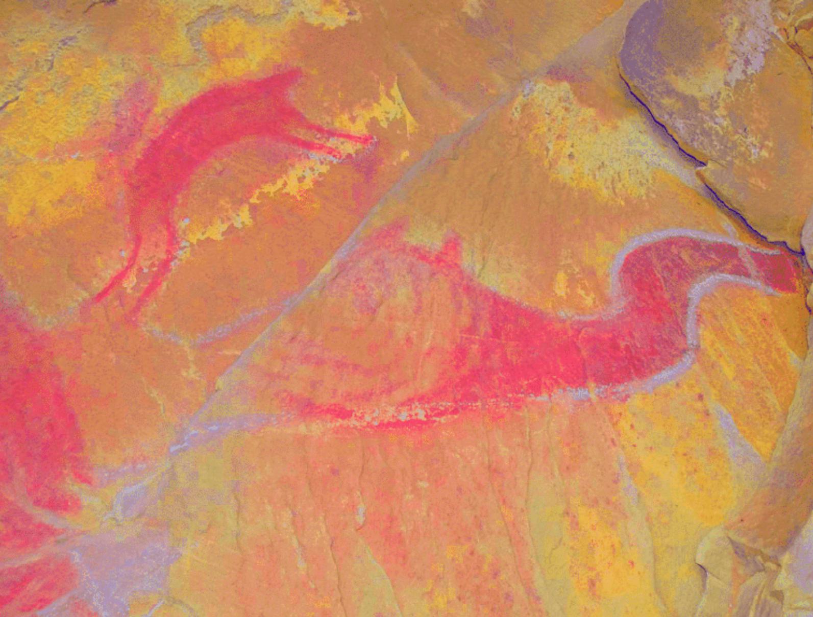
Here is my result compared with the original image:

image from paper my result

And the paper’s DStretch results:

result 2 from paper

Discussion

My result was not as clear as the paper’s due to DStretch’s additional processing techniques, but it was a fun learning experience to replicate the results of the paper at a basic level. This serves as a good example of why empirical measurement is necessary to overcome our biases and arrive at a true result. While destructive, the original chalking did attempt to figure out what the original rock art depicted. The issue with this and other subsequent attempts was since the visual information was not clear, the outlines ended up being based on interpretation instead of solid data. The 2013 paper provided a clear visual image and material composition data to provide a clearer, factual image of the original pictograph. What is concerning is that YECs still laud the Black Dragon Canyon pictograph as evidence for their fringe claims that pterosaurs were alive at the same time as humans despite the evidence. This is the most extreme example of bias, where preconceived beliefs prevent one from accepting new contrary data.

Sources

[1] “Apply decorrelation stretch to multichannel image - MATLAB decorrstretch.” https://www.mathworks.com/help/images/ref/decorrstretch.html (accessed Sep. 05, 2022).

[2] A. R. Gillespie, A. B. Kahle, and R. E. Walker, “Color enhancement of highly correlated images. I. Decorrelation and HSI contrast stretches,” Remote Sensing of Environment, vol. 20, no. 3, pp. 209–235, Dec. 1986, doi: 10.1016/0034-4257(86)90044-1.

[3] D. Dangampola, “Dhanushka Dangampola’s Blog: Decorrelation Stretching,” Dhanushka Dangampola’s Blog, Feb. 14, 2015. https://dhanushkadangampola.blogspot.com/2015/02/decorrelation-stretching.html (accessed Sep. 05, 2022).

[4] “DStretch.com home page.” http://www.dstretch.com/ (accessed Sep. 05, 2022).

[5] “lbrabec/decorrstretch: Decorrelation stretch in Python.” https://github.com/lbrabec/decorrstretch (accessed Sep. 05, 2022).

[6] J.-L. Le Quellec, P. Bahn, and M. Rowe, “The death of a pterodactyl,” Antiquity, vol. 89, pp. 872–883, Aug. 2015, doi: 10.15184/aqy.2015.54.

[7] S. Chaffee, M. Hyman, and M. Rowe, “Vandalism of Rock Art for Enhanced Photography,” Canyonlands Research Publications, vol. 39, Aug. 1994, doi: 10.1179/sic.1994.39.3.161.